Optimized Load Shedding for Voltage Resilience in Ethiopia's Power Grid

Mebratu Sintie Geremew; Yalew Gebru Workie; Joseph Ngugi Kamau; Churchill Otieno Saoke; Dessalegn Bitew Aeggegn; Gedef Yigalem Sharie

doi:doi:10.11648/j.epes.20261501.11

Research Article |

| Peer-Reviewed

Optimized Load Shedding for Voltage Resilience in Ethiopia's Power Grid

Mebratu Sintie Geremew^*

, Yalew Gebru Workie

, Joseph Ngugi Kamau

, Churchill Otieno Saoke

, Dessalegn Bitew Aeggegn

, Gedef Yigalem Sharie

Published in American Journal of Electrical Power and Energy Systems (Volume 15, Issue 1)

Received: 21 December 2025 Accepted: 4 January 2026 Published: 26 January 2026

Views: Downloads:

Download PDF

Share This Article

Twitter
Linked In
Facebook

Abstract

This study deals with the essential operational challenges of voltage instability in the Northwest Ethiopian transmission network (NETN), which is a rapidly growing energy demand. An intelligent voltage load-shedding framework, Particle Swarm Optimization, was used for the multi-objective function under contingency scenarios. The proposed method, tested on NETN, comprising 15 buses, 15 lines, two generators, and three external grids, was used to analyze the grid behavior under significant load escalation (50% and 75% increase). The results indicated severe voltage drops at critical buses, notably Metema and Gondar (Metema’s voltage declined from 0.978 p.u. to 0.8638 p.u. at 75% overload). The proposed algorithm combines voltage sensitivity indices with dynamic load-shedding logic to determine the exact place & magnitude of real power changes. PSO-based optimization simultaneously minimizes active power curtailment while maximizing voltage profile recovery. Upon activation, the strategy restored bus voltages to secure levels (Metema up to 0.9538 p.u.) with precise bus-specific shedding of real power. This method effectively and rapidly transitions the system from an emergency to a normal state with minimal load loss. In contrast to traditional approaches, this comprehensive method explores feasibility in near real-time and guarantees system-wide coordination, providing a cost-effective solution for enhancing reliability in developing power systems across various uncertainty and stress conditions. These findings provide an innovative and practical foundation for enhancing the voltage stability.

Published in	American Journal of Electrical Power and Energy Systems (Volume 15, Issue 1)
DOI	10.11648/j.epes.20261501.11
Page(s)	1-13
Creative Commons	This is an Open Access article, distributed under the terms of the Creative Commons Attribution 4.0 International License (http://creativecommons.org/licenses/by/4.0/), which permits unrestricted use, distribution and reproduction in any medium or format, provided the original work is properly cited.
Copyright	Copyright © The Author(s), 2026. Published by Science Publishing Group

Keywords

Contingency Analysis, Ethiopian Power Grid, Load Shedding, Particle Swarm Optimization, Power System Stability, Real-time Control, Voltage Sensitivity

1. Introduction

The present power system spans more than a century and has interconnected the generation stations, transmission networks, and distribution systems

[1]

. The most popular energy source in the real world, electricity, is used by a number of users in the commercial, residential, industrial, and transportation sectors. It significantly benefits society by offering vital services worldwide. When a power system runs continuously, it is considered to be stable. However, owing to various contingency conditions such as line outage, generator trip, and transformer failures, the running state varies from one operating state to another.

However, ensuring a consistent flow of electricity is crucial for contemporary life. Despite their technical sophistication, power grids are susceptible to disruptions caused by unexpected demand surges and equipment failures. These unexpected incidents, referred to as contingencies (such as lines, generators, and transformers), can lead to voltage instability and cascading outages, resulting in significant economic and social repercussions and potentially plunging the entire region into darkness. To overcome these issues, power system operators may apply intelligence-based load shedding, which involves intentionally reducing the electrical load in the requested load area. This study examined a novel load-shedding strategy that utilizes contingency analysis through the application of MPSO.

The main contributions of this study are as follows:

1) Investigate potential power outages and evaluate how they affect grid stability, particularly voltage stability.

2) Develop an optimization algorithm that utilizes a PSO-based load-shedding strategy to achieve an optimal response to contingency events.

3) Optimize the amount of power for shedding on each load bus.

4) Minimize load shedding requirement while ensuring grid stability (voltage within an acceptable limit).

Generally, this study emphasizes developing and evaluating a PSO-based load-shedding strategy to mitigate the impact of power outage conditions, such as load-increasing conditions, on grid stability, specifically voltage stability.

Researchers have considered various methodologies to establish technical load shedding systems. The following section provides an overview of the diverse approaches used by different researchers. Presented voltage stability for enhancing reliable power systems, particularly post-global blackouts. It mitigates the use of FACTS devices to manage reactive power compensation for rising loads. The authors determined the optimal locations for static var compensators using PV/QV curves and SVS assessments, with simulations conducted using the DigSilent Power Factory simulator

[2, 3]

Anticipated a new UFLS design that uses power electronics instead of conventional relays to control the load more smoothly. This can improve the efficiency of UFLS by enabling near real-time modifications depending on the frequency deviation index. Through simulations, the authors examined and contrasted these approaches with other UFLS techniques, with a particular emphasis on under-frequency problems

[4]

Pourghasem and Seyedi suggested a novel technique called UVLS to stop voltage collapse in microgrids, which are being utilized more and more as independent power sources. To ensure system stability, the technique ranks and disconnects essential loads using a voltage stability index. The authors used DIgSILENT PowerFactory software to simulate a microgrid using wind, solar, and microturbine power sources in order to test their methodology

[5]

Usman Proposed a UVLS system that reduces load shedding expenses, voltage variation, and power loss. A sophisticated "evolutionary particle swarm optimization" method efficiently establishes the ideal load shedding level. The IEEE-33 bus system was used for testing, and the researchers found that their approach outperformed conventional PSO algorithms in identifying the best answers

[6]

Cruz Suggested a novel technique for enhancing load curtailment control in medium voltage distribution systems that makes use of particle swarm optimization (PSO). PSO seeks to reduce the necessity of real load shedding. PSO enables effective online control of the load curtailment issue since it is well-suited for real-time deployment. Security limitations based on system element voltage and loading limits are taken into account during optimization

[7]

Mogaka examined the effects on islanded microgrids of a substantial incorporation of renewable energy sources. The study uses a standard IEEE 30-bus system on the MATLAB platform to examine both generation and overload issues. The Artificial Bee Colony algorithm is used in the study to maximize load shedding. The outcomes are contrasted with those generated by the GA-PSO hybrid approach, Particle Swarm Optimization, and Genetic Algorithm

[8]

Hafez suggested a novel method for power grids called Under-Frequency Load Shedding (UFLS) that makes use of Multi-Objective Particle Swarm Optimization (MOPSO). In order to create a more reliable and effective UFLS system, MOPSO seeks to minimize load shedding while optimizing the minimum system frequency. Using MATLAB and DIgSILENT PowerFactory software, the researchers evaluated MOPSO against different optimization methods, including adaptive and classic ones, on IEEE bus systems

[9]

Even though load shedding and voltage stability augmentation have been studied extensively, existing approaches have a number of drawbacks in high-stress, real-world operating scenarios. Reactive power management is the main goal of approaches that use FACTS devices; however, they lack dynamic adaptability and necessitate expensive infrastructure. Basic threshold-based control is provided by UFLS and UVLS systems; however, they frequently react slowly to sudden spikes in load and do not maximize the quantity or location of load shedding. Although heuristic approaches like basic PSO and Genetic Algorithms (GA) have demonstrated promise in resolving complex power optimization issues, many of these studies either lack multi-objective coordination or fail to consider voltage sensitivity when formulating their solutions. Furthermore, there has been little investigation of region-specific topologies, such as those seen in the Ethiopian grid, and the majority of previous work has been tested on standardized IEEE systems. These shortcomings highlight the necessity of a load-shedding method that is dynamically responsive, sensitive, and computationally efficient in order to meet real-world contingency circumstances.

This study's primary contribution is the creation of a load-shedding method based on Modified Particle Swarm Optimization (PSO) that is specifically intended to improve voltage stability in power systems during emergencies. The suggested approach presents a voltage-sensitivity guided optimization framework that dynamically determines the location and magnitude of real power to be shed across the network, in contrast to traditional strategies that either apply fixed shedding thresholds or optimize without sensitivity coordination. Multi-objective optimization routines that concurrently decrease the overall load shed and restore voltage profiles within allowable operating limits are embedded to accomplish this.

In addition to changing the PSO algorithm, the approach is new because it carefully incorporates voltage sensitivity indices into the fitness assessment procedure, which enables the system to give priority to shedding from buses that have the most stability impact. This allows for targeted, minimal, and quick corrective operations and makes the system extremely sensitive to severe load disruptions. Two major contingency scenarios that are reflective of high-stress grid conditions, 50% and 75% increases in load demand, have been used to evaluate the approach. The algorithm's resilience and usefulness were demonstrated in both situations when it successfully restored the power levels of vital buses like Metema and Gondar. The technique is particularly pertinent for developing power systems with low infrastructural resilience, like those in the Ethiopian grid, because it is computationally lightweight, scalable, and appropriate for real-time or near-real-time implementation. This study thus offers a significant methodological advancement with direct application potential for power system operators, planners, and stability control systems in regions facing volatile demand and constrained infrastructure.

2. Methods and Data Analysis

Ethiopian Electric Power delivers the most recent and significant information on information regarding generator, load, and transmission networks

[10]

. The Northwest Region transmission system's network diagram is illustrated in Figure 1 using DIgSILENT PowerFactory software. The assessment of the current condition of the power system typically initiates analysis of Newton-Raphson load flow, centered around a selected area.

Download: Download full-size image

Figure 1. Ethiopia's Northwest Electric Power Network.Ethiopia's Northwest Electric Power Network.

2.1. Load Flow Analysis of the System

Load flow analysis is probably the most important of all network calculations. Complete information about the examined system, including the rated values of the generator, transformers, lines, and values of each load's actual and reactive power, must be provided to undertake a load flow study as shown in Figure 2. It is extremely important for all network-related computations because it pertains to the network's performance under steady-state operating conditions.

Download: Download full-size image

Figure 2. Load flow analysis.Load flow analysis.

Since load flow is a non-linear problem, one can use any of the following strategies to solve it iteratively: the Newton-Raphson, rapid decoupling, and Gauss-Seidel methods. The Newton-Raphson approach, which has a faster convergence rate and is therefore more applicable to large power systems, is used in this study. The Newton-Raphson method is also a good choice for computer calculations.

Figure 3 shown below, indicates the net power injected.

Download: Download full-size image

Figure 3. Net Power injected.Net Power injected.

The system voltages V and current injection sites I's relationship is described by the nodal network equation that is created, as illustrated in the equation for a network with n buses.

Y = [\begin{matrix} Y 11 & \dots & Y 1 n \\ ⋮ & ⋱ & ⋮ \\ Yn 1 & \dots & Ynn \end{matrix}]

(1)

[\begin{matrix} I 1 \\ ⋮ \\ Ii \\ ⋮ \\ In \end{matrix}] = [\begin{matrix} Y 11 & \dots & Y 1 i \dots & Y 1 n \\ ⋮ & \dots & ⋮ & ⋮ \\ Yi 1 & \dots & Yii & \dots \\ ⋮ & \dots & ⋮ & ⋮ \\ Yni & \dots & \dots & Ynn \end{matrix}]

(2)

The values of diagonal elements (Yii) equal the total amount of admittances connected to bus I. The Yij off-diagonal elements are equivalent to the opposite side of the entry between buses I and J. Notably, for large systems, the Y-bus is a sparse matrix.

\begin{matrix} Yii = \sum_{\begin{matrix} j = 0 \\ j \neq i \end{matrix}}^{n} yij \\ Yij = Yji = - yij \end{matrix}\}

(3)

As illustrated in Figure 3, the voltage of the bus (Vi), the surrounding voltages in buses (Vj), and the admittances between the bus and its neighboring buses (yij) can all be used to determine the net injected power at any bus.

I_{i} = V_{I} (y_{i 0} + y_{i 1} + y_{i 2} + \dots \dots + y_{ij}) - V_{1} y_{i 1} + V_{2} y_{i 2} - . . . . . . . - V_{j} y_{ij}

I_{i} = V_{i} \sum_{j = 0, j \neq i} Y_{ij} - \sum_{j = 1, j \neq i} Y_{ij} V_{j} = V_{i} Y_{ii} \sum_{j = 1, j \neq i} Y_{ij} V_{j}

The power equation for any bus can be written like this:

S_{i} = P_{i} + j Q_{i} = V_{i} I_{i}^{*} or S_{i}^{*} = P_{i} - j Q_{i} = V_{i}^{*} I_{i}

(4)

\begin{matrix} Pi = \sum_{j = 1}^{n} |Vi| |Vj| |Yij| \cos ({θ_{ij} - δ}_{i} {+ δ}_{j}) \\ Qi = - \sum_{j = 1}^{n} |Vi| |Vj| |Yij| \sin (θ_{ij} - δ_{i} {+ δ}_{j}) \end{matrix}\}

(5)

2.2. Security-Related Functions

To discuss security-related functions, first, it is better to define certain quantities related to power System security

[11]

. Figure 4 shows the power system's operating state. As it starts from the top down, it is expected that the real-time data provides the current state of the power system.

Download: Download full-size image

Figure 4. functioning state of the power system.functioning state of the power system.

Normal State: At this point, no equipment is being overloaded, and all system variables are within their typical range. Such as all bus voltages are within specified limits.

Alert State: If the security level drops below a predetermined threshold for sufficiency. In this state, all system variables are still within an acceptable range, and all constraints are satisfied. Nevertheless, the system has been compromised to the point where unexpected events could result in equipment overload.

Emergency State: The system enters this state when a sufficiently severe disruption occurs in the system. Many buses have low voltage or equipment loads that are higher than the short-term emergency rating.

Restorative State: When all of the system loads are not being satisfied, the power system is in a restorative mode. It suggests a system shutdown, either complete or partial. Restoring system loads as quickly as feasible is the primary goal of this study.

Table 1 outlines the voltage thresholds used to evaluate system security under different operational states. In the alarm state, bus voltages are permitted to deviate slightly from nominal values, with a range of 0.95 to 1.05 p.u., while in the security (emergency) state, the acceptable voltage range is extended to 0.90 p.u. – 1.10 p.u. These thresholds serve as critical indicators for system operators to identify the onset of instability and to initiate remedial measures, like load shedding, before the system transitions into an emergency or restorative state.

Table 1. Alarm and security limits.Alarm and security limits.Alarm and security limits.

Parameters	Alarm limit	Security limit
Voltage of the bus (lower) (P.u)	0.95	0.9
Voltage of the bus (upper) (P.u)	1.05	1.10

2.3. Analysis of Stability for Electrical Power Systems

Electrical power system stability is the electrical power system’s ability to return to a balanced condition after disturbance

[12]

. The capacity and load of the electrical system will fluctuate at any time as it operates. The generator had to modify its ability to produce load power as a result of that adjustment, using the governor and excitation control.

2.3.1. Stability of Voltage

Voltage stability is the ability of the power system to keep each bus's voltage stable in the wake of a disturbance

[13, 14]

. The primary reason why voltage instability occurs is unbalanced reactive power. This imbalance primarily manifests itself in a system's local bus or local network. As a result, there must be enough local reactive power support. As demonstrated in Figure 5 below, as the PV curve of power versus power rises, the voltage at the power transfer's receiving end falls. Apply voltage sensitivity analysis with the UVLS approach to enhance these voltage profiles.

Download: Download full-size image

Figure 5. A power vs voltage plot.A power vs voltage plot.

2.3.2. Computational Intelligent Load Shedding

Load shedding is a protection scheme used in a power system to avoid the condition of overloading during a large disturbance. It can alter the power usage of a certain load bus and help to prevent system instability. Numerous researchers have created various load-shedding and restoration techniques, including conventional, adaptive, and computational, as shown in Figure 6.

Download: Download full-size image

Figure 6. Categorization of load-shedding methods.Categorization of load-shedding methods.

An intelligent load-shedding scheme takes into account the operating conditions before and after a disturbance, its nature, duration, the system's transient reaction to the disturbance, and the mode of users online. For extremely non-linear issues, techniques like neural networks, genetic algorithms, particle swarm optimization, simulated annealing, fuzzy logic, and others provide efficient problem-solving, knowledge representation, planning, and action

[15]

. In this condition, the mode of utilization is online.

2.3.3. Load Shedding

To make the system more functional when there are low voltage conditions, load shedding is set up. Systems that have had a disturbance may remain stable after the disturbance, although bus voltages are still low. Systems that have had a disturbance may remain stable after the disturbance, although bus voltages are still low. When voltages are too close to stability limits, collapse can occur suddenly and easily, even with voltage adjustment techniques.

Therefore, during a disturbance, the voltage may begin to fall below acceptable levels. Calculating the total power differential between the before and after conditions is the first phase of the procedure. Once the size of the disturbance has been determined, the position and the amount of load to be shed from the load bus must be decided. The next step is to calculate how much load each bus should be able to handle. The voltage sensitivity of each bus determines that. Assume that there is a single generator, transmission line, and load in a two-bus system as depicted in Figure 7 to explain sensitivity analysis.

Download: Download full-size image

Figure 7. Model representation of two buses.Model representation of two buses.

The equations are as follows when further simplified for a two-bus system:

\begin{matrix} P_{12} = |V_{1} |^{2} G - |V_{1}|| V_{2} | G^{*} \cos (δ_{12}) + | V_{1} | | V_{2} | B^{*} \sin {(δ}_{12}) \\ Q_{12} = |V_{1} |^{2} B - |V_{1}|| V_{2} | B^{*} \cos (δ_{12}) + | V_{1} | | V_{2} | G^{*} \sin {(δ}_{12}) \end{matrix}\}

(6)

The power delivered at the receiving end is now PD = -P12 and QD = -Q12. This only applies to two-bus systems; a larger system would follow a different set of steps. After the formula between QD and V2 has been formed, the previous equation can be differentiated, Eq. (6). We get,

\frac{{dQ}_{d}}{{dV}_{2}} = V_{2} * BCOS δ_{12} + V_{2} * Gsin δ_{12}

(7)

The generalized equation for the n-bus system is,

\frac{{dQ}_{i}}{{dV}_{i}} = \sum_{j = 1}^{n} |V_{j}| |Y_{ij}| \sin ({θ_{ij} - δ}_{ij})

(8)

The dQ/dV relation can be expressed as follows for each bus separately:

\begin{matrix} \frac{{dQ}_{1}}{{dV}_{1}} = \sum_{j = 1}^{n} |V_{j}| |Y_{1 j}| \sin (θ_{1 j} - δ_{1 j}) \\ \frac{{dQ}_{2}}{{dV}_{2}} = \sum_{j = 1}^{n} |V_{j}| |Y_{2 j}| \sin ({θ_{2 j} - δ}_{2 j}) \\ \frac{{dQ}_{n}}{{dV}_{n}} = \sum_{j = 1}^{n} |V_{j}| |Y_{nj}| \sin (θ_{nj} - δ_{nj}) \end{matrix}\}

(9)

if load bus X's dQ/dV value is greater than load bus Y's dQ/dV value. Therefore, a higher load must be released from lower levels of dQ/dV. Thus,

\frac{{dQ}_{i}}{{dV}_{i}}  (\frac{1}{The} amount of load that each bus must shed)

To assess this load quantity, take the reciprocal of the voltage sensitivity as a percentage of the total reciprocal of the voltage sensitivities.

\frac{dV}{dQ} = (1 / \frac{dQ}{dV})

(10)

\frac{{dV}_{i}}{{dQ}_{i}} = (1 / \sum_{j = 1}^{n} |V_{j}| |Y_{ij}| \sin ({θ_{ij} - δ}_{ij})

(11)

For each bus, the equation above provides a value that is fractional for the voltage sensitivity. The amount of load that needs to be shed, as well as the dV/dQ value at every bus, is now directly related.

\frac{{dV}_{i}}{{dQ}_{i}}  (amount of load that each bus must shed)

The aggregate of all the buses' dV/dQ values is now,

\sum_{i = 1}^{n} \frac{{dV}_{i}}{{dQ}_{i}} = \frac{{dV}_{1}}{{dQ}_{1}} + \frac{{dV}_{2}}{{dQ}_{2}} + \dots \frac{{dV}_{n}}{{dQ}_{n}}

(12)

The equation above adds together the dV/dQ values at each load bus. In order to keep the power balance, less load must be discharged overall than at each bus. The fraction of the dV/dQ value at each bus that corresponds to the previously calculated total is the load percentage at each bus. This is shown as

\frac{\frac{{dV}_{i}}{{dQ}_{i}}}{(\frac{{dV}_{1}}{{dQ}_{1}} + \frac{{dV}_{2}}{{dQ}_{2}} + \dots \frac{{dV}_{n}}{{dQ}_{n}}}

(13)

This represents a fraction of all voltage sensitivity. Therefore, the load that each bus must drop is determined depending on the bus's proximity to the knee point when this percentage is multiplied by the entire load that needs to be shed.

The empirical formula that will be examined is;

Si = \frac{\frac{{dV}_{i}}{{dQ}_{i}}}{(\frac{{dV}_{1}}{{dQ}_{1}} + \frac{{dV}_{2}}{{dQ}_{2}} + \dots \frac{{dV}_{n}}{{dQ}_{n}}} Pdiff

(14)

This equation determines the necessary power shedding for each load bus during load conditions. This calculation provides a precise value for the power that needs to be shed at each location. It is done by leveraging Equation (13), the voltage sensitivity factor of the bus, and multiplying it by the power difference (Pdiff) at each bus. This calculation provides a precise value for the power that needs to be shed at each location.

2.3.4. Particle Swarm Optimization

PSO was introduced by Kennedy and Eberhart in 1995

[9]

. PSO is a member of the class of swarm intelligence approaches designed to address large-scale non-linear optimization issues. The social behavior of animals, such as fish schools and flocks of birds, served as its inspiration. PSO is a powerful meta-heuristic search technique.

PSO has the following benefits over other artificial intelligence systems

[16]

: PSO uses competition and teamwork to decide on the next step's direction. Compared to the simulated Annealing method and the Genetic Algorithm method, fewer parameters need to be set. The complexity of the objective functions has less of an impact on PSO's calculation time. The overall graphical representation of PSO is shown in Figure 8 below.

Download: Download full-size image

Figure 8. Graphical Illustration of the PSO Algorithm.Graphical Illustration of the PSO Algorithm.

V_{id}^{(k + 1)} = w * V_{id}^{(k)} + C_{1} r_{1} (P_{id}^{Best} - X_{id}^{(k)}) + C_{2} r_{2} (G_{d}^{best} - X_{id}^{k})

(15)

X_{id}^{(k + 1)} = X_{id}^{(k)} + V_{id}^{(k + 1)}

(16)

2.4. Problem Formulation

The following are the two primary goals of the under-voltage shedding system:

To reduce the overall load shed on the chosen buses.

To minimize voltage drops at all buses.

This optimization problem can be formalized as follows.

2.4.1. Objective Function

F_{objective} = \min {f 1, f 2}

(17)

The equation represents the multi-objective function for power shedding in the load bus and voltage profile change. The optimization algorithm determines the amount of power shedding by minimizing the objective functions.

Where f1 and f2 are the objective functions used to identify the power shed for each bus and voltage profile change, respectively. The proposed strategy aims to minimize the load shedding value while optimizing the power system's voltage stability.

The following mathematical formulation of f1 and f2, listed in equation (18), is used to define the individual objective function. This is crucial for voltage stability and load shedding when using the PSO algorithm.

\begin{matrix} f 1 = Si \\ f 2 = \sum_{i \in N_{bus}} |1 - Vi| \end{matrix}\}

(18)

2.4.2. Constraints

The optimization issue requires consideration of both equality and inequality constraints.

1) Equality Constraints

Equations for the balance of reactive and real power can be expressed in equality constraints.

\begin{matrix} P_{ij} = \sum_{j = 1} ViVj (G_{ij} \cos θ_{ij} + B_{ij} \sin θ_{ij}) where i ϵ N_{bus} \\ Q_{ij} = \sum_{j = 1} ViVj (G_{ij} \sin θ_{ij} - B_{ij} \cos θ_{ij}) where i ϵ N_{bus} \end{matrix}\}

(19)

2) Inequality Constraints

The minimum and maximum bus voltage magnitude, real, and reactive power range during generation bus injection are the inequality constraints.

\begin{matrix} P_{i}^{\min} \leq P_{i} \leq P_{i}^{\max}, i ϵ B_{gen} \\ Q_{i}^{\min} \leq Q_{i} \leq Q_{i}^{\max}, i \in B_{gen} \\ V_{i}^{\min} \leq V_{i} \leq V_{i}^{\max}, i \in N_{bus} \end{matrix}\}

(20)

2.5. Load Shedding Algorithm of Particle Swarm Optimization

Step 1: For a power outage, use the complete A. C. Newton-Raphson power flow.

Step 2: Find out the load bus's sensitivity factor.

Step 3: Consider the sensitivity factors and then calculate the rate of disturbance that will occur in each bus.

Step 4: Construct a population of randomly generated particles as a reference point.

Step 5: Fitness determines each particle's fitness.

Step 6: By comparing each particle's current pbest fitness, update each particle's individual best solution (pbest).

Step 7: Update the new particle positions and velocities using equations (15) and (16).

Step 8: Find the updated global best solution by evaluating each particle's new fitness value in light of its changed position and velocity. Additionally, modify the Pbest and Gbest values.

Step 9: Generate a new population.

Step 10: Until the convergence condition is met, go to step 7.

Step 11: Stop the simulation.

3. Outputs and Discussion

3.1. The simulation's Base Case Value

With just three iterations, the Newton-Raphson load-flow simulation was gathered. Nevertheless, the network's power flow analysis operates under many circumstances.

As depicted in Figure 9, the voltage magnitude for each bus remains within the normal range under standard conditions, indicating no voltage violations. However, certain buses may experience a decrease in voltage profile below their limits during transitions from emergency to extreme states and from alert to emergency within the power system. This can be attributed to fluctuations in load or line disconnections. Consequently, conducting a contingency analysis becomes crucial to address potential security concerns.

Download: Download full-size image

Figure 9. Each bus's voltage violations in the base.Each bus's voltage violations in the base.

3.2. Scenario 1: Each Bus's Voltage Profile Under Loading Conditions

3.2.1. Simulation Result of Bus Voltage violations Before, During, and After the Load Shedding System for a 1.5 Load Factor

Table 2 and Figure 10 show the load bus's voltage profile data before, during, and after the load-shedding process. In a typical scenario, load buses 8 and 9 have voltage profiles of 0.978 and 0.961 per unit, respectively, as shown in the figure below. But with a 50% state of rising load, their voltage profile has decreased to 0.888 and 0.885 voltage per unit. The deviation in voltage profiles for Metema and Gondar load buses compared to others can be attributed to their longer distance from the generation station to the load center and their high loading rates. This underscores the significant impact of unplanned load variations on each load bus's unique voltage profile. However, its voltage profile restored to normal after load shedding was implemented.

Table 2. Bus voltage of the 15 bus system in Normal, during contingency (Load Factor 1.5), and after load shed.Bus voltage of the 15 bus system in Normal, during contingency (Load Factor 1.5), and after load shed.Bus voltage of the 15 bus system in Normal, during contingency (Load Factor 1.5), and after load shed.

Voltage in per unit
Bus No	Bus name	Normal base	During loading (50%)	Load shed for 50% By PSO
1	Belesin	1.000	1.0500	1.0500
2	Tissin	1.000	1.0000	1.0000
3	Belesout	0.999	1.0100	1.0300
4	Tissout	0.987	0.9700	0.9900
5	BDII230	0.991	0.9564	0.9829
6	D/M400	0.999	0.9900	1.0100
7	D/M230	0.990	0.9702	0.9917
8	Metema	0.978	0.8879	0.9538
9	GOII	0.961	0.8849	0.9523
10	N/Mew	0.994	0.9549	0.9846
11	Gashena	0.995	0.9859	0.9911
12	Alamata	1.000	0.9900	0.9900
13	Motta	0.994	0.9610	0.9869
14	Fincha	1.000	0.9700	0.9900
15	Sululita	1.000	1.0000	1.0200

Download: Download full-size image

Figure 10. Magnitudes of voltage (PU) base case, load, and Shedd after LF 1.5. Magnitudes of voltage (PU) base case, load, and Shedd after LF 1.5.

3.2.2. Simulation Result of Bus Voltage Violations Before, During, and After the Load Shedding System for a 1.75 Load Factor

Table 3 and Figure 11 show the load bus's voltage profile results before, during, and after the load-shedding process. As observed in Figure 11, the voltage profile of load bus 8 and load bus 9 in a normal case is 0.978 and 0.961 per unit, respectively. But with a 75% load-increasing condition, their voltage profile has decreased to 0.863 and 0.860 voltage per unit. The reason why the voltage profiles of Metema and Gondar load buses are lower than those of others. Because of their longer distance from the generation station to the load center and their high loading rates. This underscores the significant impact of unplanned load variations on the voltage profiles of individual load buses. But after taking load-shedding action, its voltage profile returned to normal condition.

Table 3. Bus voltage of 15 bus systems in Normal, during contingency (1.75 Load Factor), and after load shed.Bus voltage of 15 bus systems in Normal, during contingency (1.75 Load Factor), and after load shed.Bus voltage of 15 bus systems in Normal, during contingency (1.75 Load Factor), and after load shed.

Voltage in per unit
Bus No	Bus name	Normal base	During loading (75%)	Load shed for 75% By PSO
1	Belesin	1.000	1.0500	1.0500
2	Tissin	1.000	1.0000	1.0000
3	Belesout	0.999	1.0100	1.0300
4	Tissout	0.987	0.9700	0.9700
5	BDII230	0.991	0.9469	0.9697
6	D/M400	0.999	0.9900	1.0100
7	D/M230	0.990	0.9655	0.9862
8	Metema	0.978	0.8638	0.9522
9	GOII	0.961	0.8600	0.9501
10	N/Mew	0.994	0.9449	0.9719
11	Gashena	0.995	0.9835	0.9884
12	Alamata	1.000	0.9900	0.9900
13	Motta	0.994	0.9536	0.9777
14	Fincha	1.000	0.9700	0.9900
15	Sululita	1.000	1.0000	1.0000

Download: Download full-size image

Figure 11. Magnitudes of voltage (PU) base case, load, and Shedd at LF 1.75.Magnitudes of voltage (PU) base case, load, and Shedd at LF 1.75.

3.3. Scenario 2: Load Bus Real Power Magnitude During Loading Condition

3.3.1. Load Bus Real Power Magnitude Before, During, and After the Load Shedding System for a 1.5 Load Factor

In the conducted test system, comprising 2 generators, 15 buses, and 15 transmission lines, the load-shedding technique focuses primarily on managing load variability at the load bus. The methodology involves inducing loading on the load bus, followed by the application of load shedding to determine how much power each load bus needs to be reduced.

The outputs and discussion present Table 4 and Figure 12, illustrating the load bus's actual power magnitude in normal conditions, during contingency, and after executing the load-shedding system. When the demand for the load bus increases by 50%, the bus's real power magnitude is trending increasing. However, following the load-shedding intervention, the real power magnitude of the load bus experiences a decrease. As shown in Table 4, the BDII230 load bus typically has a load of 0.8823 per unit. However, the load increased by 50% its real power magnitude was updated from 0.8823 to 1.3235 per unit. But after taking load shedding action real power magnitude decreased from 1.3235 to 0.8958 per unit. Similarly, the remaining load bus has decreased by such an amount of power.

Table 4. Real power of the load bus in normal, during contingency (1.5 Load Factor), and after load shed.Real power of the load bus in normal, during contingency (1.5 Load Factor), and after load shed.Real power of the load bus in normal, during contingency (1.5 Load Factor), and after load shed.

Load power in per unit
Load Bus No	Bus Name	Normal case (MW)	During loading(50%) (MW)	Load shed for 50% PSO(MW)
5	BDII230	0.8823	1.3235	0.8958
7	D/M230	0.3468	0.5202	0.3521
8	Metema	0.4981	0.7472	0.5057
9	GOII	0.0340	0.0510	0.0345
10	N/Mew	0.0847	0.1271	0.0860
11	Gashena	0.1000	0.1500	0.1015
13	Motta	0.0667	0.1001	0.0667

Download: Download full-size image

Figure 12. Load power (PU) base case, load, and Shedd at LF1.5.Load power (PU) base case, load, and Shedd at LF1.5.

3.3.2. Load Bus Real Power Magnitude Before, During, and After the Load Shedding System for a 1.75 Load Factor

The results and discussion present Table 5 and Figure 13, illustrating the load bus's actual power magnitude in normal conditions, during emergencies, and after executing the load-shedding system. When the demand for the load bus increases by 75%, the bus's real power magnitude is trending increasing. However, following the load-shedding intervention, the real power magnitude of the load bus experiences a decrease. As shown in Table 5, the BDII230 load bus typically has a load of 0.8823 per unit. However, the load increased by 75%, and its real power magnitude was updated from 0.8823 to 1.5440 per unit. But after taking load shedding action real power magnitude decreased from 1.5440 to 1.0451 per unit. Similarly, the remaining load bus has decreased by such an amount of power.

Table 5. Real power of the load bus in normal, during contingency (1.75 Load factor), and after load shed.Real power of the load bus in normal, during contingency (1.75 Load factor), and after load shed.Real power of the load bus in normal, during contingency (1.75 Load factor), and after load shed.

Load power in per unit
Load Bus No	Load Bus Name	Normal case (MW)	During loading (75%) MW	Load shed for 75% PSO(MW)
5	BDII230	0.8823	1.5440	1.0451
7	D/M230	0.3468	0.6069	0.4108
8	Metema	0.4981	0.8717	0.5900
9	GOII	0.0340	0.0595	0.0403
10	N/Mew	0.0847	0.1482	0.1003
11	Gashena	0.1000	0.1750	0.1183
13	Motta	0.0667	0.1167	0.0790

Download: Download full-size image

Figure 13. Load power (PU)base case, load, and Shedd at LF 1.75.Load power (PU)base case, load, and Shedd at LF 1.75.

4. Conclusion

This paper presents the critical impacts of voltage instability in systems under various disturbance conditions to consider scenarios with sudden load variations. The proposed algorithm is an MPSO-based load-shedding algorithm that is validated as an effective strategy for enhancing the system reliability and operational stability in a 15-bus test system representative of the NETN. The performance of the algorithm under a multi-objective function includes power shedding in the load bus and voltage profile changes, particularly in power systems with limited infrastructure flexibility. Its capability to adapt to varying load conditions and identify defined corrective actions underscores its applicability in contingency management and dynamic stability enhancement. Loading by 50% and 75% is considered a severe voltage depression at critical buses, including Metema and Gondar, and contributes to the overload conditions across several transmission lines. The proposed framework successfully mitigated these issues by accurately determining where and how much real power should be shed using a combination of voltage sensitivity indices and multi-objective optimization criteria. This approach not only reduces the extent of the load curtailment but also restores bus voltages to within permissible operating thresholds, thereby preventing voltage collapse. Although the proposed methodology has proven effective in a given test system, future research should consider integrating intermittent renewable energy sources, which also suggests uncertainty and optimal control strategies. Furthermore, developing a real-time implementation framework and validating the algorithm on large-scale interconnected power systems are important for assessing its scalability, robustness, and practical feasibility.

Abbreviations

EEP	Ethiopia Electric Power
FACTs	Flexible Alternating Current Transmission System
NETN	Northwest Ethiopian Transmission Network
PSO	Particle Swarm Optimization
UFLS	Under Frequency Load Shedding
UVLS	Under Voltage Load Shedding

Author Contribution

Mebratu Sintie Geremew: Conceptualization, Data curation, Formal Analysis, Investigation, Methodology, Resources, Software, Supervision, Visualization, Writing original draft, Writing – review & editing

Yalew Gebru Werkie: Conceptualization, Data curation, Formal Analysis, Investigation, Methodology, Resources, Software, Supervision, Visualization, Writing original draft, Writing – review & editing.

Joseph Ngugi Kamau: Formal Analysis, Supervision, Validation, Visualization, Writing – original draft, Writing review & editing

Churchill Otieno Saoke: Formal Analysis, Supervision, Validation, Visualization, Writing – original draft, Writing review & editing

Dessalegn Bitew Aeggegn: Formal Analysis, Supervision, Validation, Visualization, Writing – original draft, Writing –review & editing

Gedef Yigalem Sharie: Formal Analysis, Supervision, Validation, Visualization, Writing – original draft, Writing –review & editing

Conflicts of Interest

Authors stated that no conflict of interest.

References

[1]	R. York and S. E. Bell, “Energy transitions or additions?: Why a transition from fossil fuels requires more than the growth of renewable energy,” Energy Res. Soc. Sci., vol. 51, no. November 2018, pp. 40-43, 2019, [Online]. Available: https://doi.org/10.1016/j.erss.2019.01.008
[2]	N. Manjul and M. S. Rawat, “PV/QV Curve based Optimal Placement of Static Var System in Power Network using DigSilent Power Factory,” 8th IEEE Power India Int. Conf. PIICON 2018, no. July 2020, pp. 1-6, 2018, https://doi.org/10.1109/POWERI.2018.8704441
[3]	M. S. Geremew, Y. G. Workie, and L. B. Techane, “Identification of System Exposure for the Northwest Region of Ethiopian Electric Power,” Iran. J. Sci. Technol. Trans. Electr. Eng., vol. 0123456789, 2024, [Online]. Available: https://doi.org/10.1007/s40998-024-00698-x
[4]	Y. Yang and R. Li, “Techno-economic optimization of an off-grid solar/wind/battery hybrid system with a novel multi-objective differential evolution algorithm,” Energies, vol. 13, no. 7, pp. 1-16, 2020, https://doi.org/10.3390/en13071585
[5]	P. Pourghasem and H. Seyedi, “An under-voltage load shedding scheme to prevent voltage collapse in a microgrid,” Int. Conf. Prot. Autom. Power Syst. IPAPS 2019, no. February, pp. 12-16, 2019, https://doi.org/10.1109/IPAPS.2019.8641952
[6]	M. Usman, A. Amin, M. M. Azam, and H. Mokhlis, “Optimal Under Voltage Load Scheme for a Distribution Network Using EPSO Algorithm,” no. September 2019, 2018, https://doi.org/10.1109/ICPESG.2018.8384525
[7]	L. M. Cruz, D. L. Alvarez, A. S. Al-Sumaiti, and S. Rivera, “Load curtailment optimization using the PSO algorithm for enhancing the reliability of distribution networks,” Energies, vol. 13, no. 12, 2020, https://doi.org/10.3390/en13123236
[8]	O. Mogaka, R. Orenge, and J. Ndirangu, “Static Voltage Stability Assessment of the Kenyan Power Network,” J. Electr. Comput. Eng., vol. 2021, https://doi.org/10.1155/2021/5079607
[9]	A. A. Hafez et al., “Multi-Objective Particle Swarm for Optimal Load Shedding Remedy Strategies of Power System,” Electr. Power Components Syst., vol. 0, no. 0, pp. 1-16, 2019.
[10]	EEP, “Ethiopian Power System Expansion Master Plan Study,” 2014.
[11]	A. N. J. B. P. Kundur, Power system stability and control, vol. 7. 1994.
[12]	I. B. S, A. Nurdiansyah, A. Lomi, A. E. Power, and S. Stability, “Impact of Load Shedding on Frequency and Voltage System,” IEEE, pp. 110-115, 2017, https://doi.org/10.1109/ISITIA.2017.8124064
[13]	S. S. Refaat, H. Abu-Rub, A. P. Sanfilippo, and A. Mohamed, “Impact of grid-tied large-scale photovoltaic system on dynamic voltage stability of electric power grids,” IET Renew. Power Gener., vol. 12, no. 2, pp. 157-164, 2018, https://doi.org/10.1049/iet-rpg.2017.0219
[14]	M. S. Geremew, Y. G. Workie, J. N. Kamau, M. Bajaj, and L. B. Techane, “Voltage Stability Enhancement in North West Ethiopia ’ s Power Grid Using Contingency Analysis and PSO-Based Load Shedding,” vol. 11, no. 3, pp. 41-58, 2025, https://doi.org/10.11648/j.ajme.20251103.11
[15]	H. Haes, M. Esmail, H. Golshan, T. Cuthbert, and N. D. Hatziargyriou, “An Overview of UFLS in Conventional, Modern, and Future Smart Power Systems : Challenges and Opportunities,” Electr. Power Syst. Res., vol. 179, no. February 2019, p. 106054, 2020, https://doi.org/10.1016/j.epsr.2019.106054
[16]	S. Acharya, I. Sahoo, J. Senapati, A. Agarwal, P. Mishra, and R. K. Dash, “Performance Analysis of the PSO Algorithm: An Experimental Study,” SSRN Electron. J., no. January, 2021, https://doi.org/10.2139/ssrn.3850129

Cite This Article

Plain Text BibTeX RIS

APA Style

Geremew, M. S., Workie, Y. G., Kamau, J. N., Saoke, C. O., Aeggegn, D. B., et al. (2026). Optimized Load Shedding for Voltage Resilience in Ethiopia's Power Grid. American Journal of Electrical Power and Energy Systems, 15(1), 1-13. https://doi.org/10.11648/j.epes.20261501.11

Copy | Download

ACS Style

Geremew, M. S.; Workie, Y. G.; Kamau, J. N.; Saoke, C. O.; Aeggegn, D. B., et al. Optimized Load Shedding for Voltage Resilience in Ethiopia's Power Grid. Am. J. Electr. Power Energy Syst. 2026, 15(1), 1-13. doi: 10.11648/j.epes.20261501.11

Copy | Download

AMA Style

Geremew MS, Workie YG, Kamau JN, Saoke CO, Aeggegn DB, et al. Optimized Load Shedding for Voltage Resilience in Ethiopia's Power Grid. Am J Electr Power Energy Syst. 2026;15(1):1-13. doi: 10.11648/j.epes.20261501.11

Copy | Download

@article{10.11648/j.epes.20261501.11,
  author = {Mebratu Sintie Geremew and Yalew Gebru Workie and Joseph Ngugi Kamau and Churchill Otieno Saoke and Dessalegn Bitew Aeggegn and Gedef Yigalem Sharie},
  title = {Optimized Load Shedding for Voltage Resilience in Ethiopia's Power Grid},
  journal = {American Journal of Electrical Power and Energy Systems},
  volume = {15},
  number = {1},
  pages = {1-13},
  doi = {10.11648/j.epes.20261501.11},
  url = {https://doi.org/10.11648/j.epes.20261501.11},
  eprint = {https://article.sciencepublishinggroup.com/pdf/10.11648.j.epes.20261501.11},
  abstract = {This study deals with the essential operational challenges of voltage instability in the Northwest Ethiopian transmission network (NETN), which is a rapidly growing energy demand. An intelligent voltage load-shedding framework, Particle Swarm Optimization, was used for the multi-objective function under contingency scenarios. The proposed method, tested on NETN, comprising 15 buses, 15 lines, two generators, and three external grids, was used to analyze the grid behavior under significant load escalation (50% and 75% increase). The results indicated severe voltage drops at critical buses, notably Metema and Gondar (Metema’s voltage declined from 0.978 p.u. to 0.8638 p.u. at 75% overload). The proposed algorithm combines voltage sensitivity indices with dynamic load-shedding logic to determine the exact place & magnitude of real power changes. PSO-based optimization simultaneously minimizes active power curtailment while maximizing voltage profile recovery. Upon activation, the strategy restored bus voltages to secure levels (Metema up to 0.9538 p.u.) with precise bus-specific shedding of real power. This method effectively and rapidly transitions the system from an emergency to a normal state with minimal load loss. In contrast to traditional approaches, this comprehensive method explores feasibility in near real-time and guarantees system-wide coordination, providing a cost-effective solution for enhancing reliability in developing power systems across various uncertainty and stress conditions. These findings provide an innovative and practical foundation for enhancing the voltage stability.},
 year = {2026}
}

Copy | Download

TY - JOUR
T1 - Optimized Load Shedding for Voltage Resilience in Ethiopia's Power Grid
AU - Mebratu Sintie Geremew
AU - Yalew Gebru Workie
AU - Joseph Ngugi Kamau
AU - Churchill Otieno Saoke
AU - Dessalegn Bitew Aeggegn
AU - Gedef Yigalem Sharie
Y1 - 2026/01/26
PY - 2026
N1 - https://doi.org/10.11648/j.epes.20261501.11
DO - 10.11648/j.epes.20261501.11
T2 - American Journal of Electrical Power and Energy Systems
JF - American Journal of Electrical Power and Energy Systems
JO - American Journal of Electrical Power and Energy Systems
SP - 1
EP - 13
PB - Science Publishing Group
SN - 2326-9200
UR - https://doi.org/10.11648/j.epes.20261501.11
AB - This study deals with the essential operational challenges of voltage instability in the Northwest Ethiopian transmission network (NETN), which is a rapidly growing energy demand. An intelligent voltage load-shedding framework, Particle Swarm Optimization, was used for the multi-objective function under contingency scenarios. The proposed method, tested on NETN, comprising 15 buses, 15 lines, two generators, and three external grids, was used to analyze the grid behavior under significant load escalation (50% and 75% increase). The results indicated severe voltage drops at critical buses, notably Metema and Gondar (Metema’s voltage declined from 0.978 p.u. to 0.8638 p.u. at 75% overload). The proposed algorithm combines voltage sensitivity indices with dynamic load-shedding logic to determine the exact place & magnitude of real power changes. PSO-based optimization simultaneously minimizes active power curtailment while maximizing voltage profile recovery. Upon activation, the strategy restored bus voltages to secure levels (Metema up to 0.9538 p.u.) with precise bus-specific shedding of real power. This method effectively and rapidly transitions the system from an emergency to a normal state with minimal load loss. In contrast to traditional approaches, this comprehensive method explores feasibility in near real-time and guarantees system-wide coordination, providing a cost-effective solution for enhancing reliability in developing power systems across various uncertainty and stress conditions. These findings provide an innovative and practical foundation for enhancing the voltage stability.
VL - 15
IS - 1
ER -

Copy | Download

Author Information

Mebratu Sintie Geremew

Department of Electrical & Computer Engineering, Mizan-Tepi University, Mizan-Tepi, Ethiopia;Institute of Energy and Environmental Technology, Jomo Kenyatta University of Agriculture and Technology, Juja, Kenya

Contact Email

http://orcid.org/0009-0009-4463-9264
Yalew Gebru Workie

Faculty of Electrical and Computer Engineering, Debre Markos University, Debre Markos, Ethiopia

Contact Email

http://orcid.org/0009-0007-3045-3421
Joseph Ngugi Kamau

Institute of Energy and Environmental Technology, Jomo Kenyatta University of Agriculture and Technology, Juja, Kenya

Contact Email

http://orcid.org/0000-0002-5298-4457
Churchill Otieno Saoke

Institute of Energy and Environmental Technology, Jomo Kenyatta University of Agriculture and Technology, Juja, Kenya

Contact Email

http://orcid.org/0000-0002-3014-318X
Dessalegn Bitew Aeggegn

Faculty of Electrical and Computer Engineering, Debre Markos University, Debre Markos, Ethiopia

Contact Email

http://orcid.org/0000-0002-7253-1287
Gedef Yigalem Sharie

School of Electrical and Computer Engineering, Woldia University, Woldia, Ethiopia

Contact Email

http://orcid.org/0009-0009-8711-7773

Download PDF

Submit an Article

Figure 1

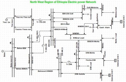
Figure 1. Ethiopia's Northwest Electric Power Network.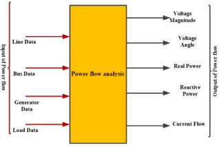
Figure 2

Figure 2. Load flow analysis.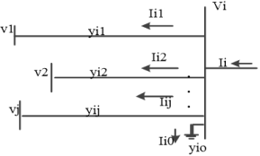
Figure 3

Figure 3. Net Power injected.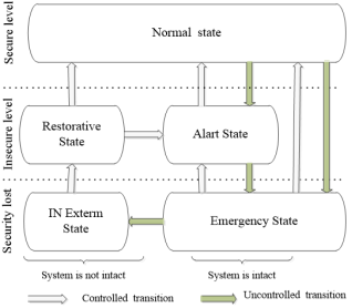
Figure 4

Figure 4. functioning state of the power system.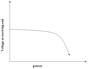
Figure 5

Figure 5. A power vs voltage plot.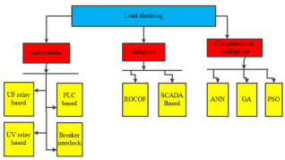
Figure 6

Figure 6. Categorization of load-shedding methods.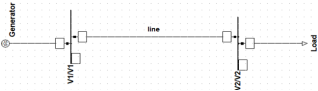
Figure 7

Figure 7. Model representation of two buses.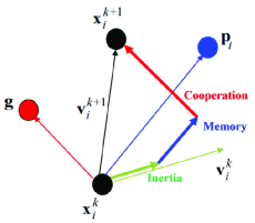
Figure 8

Figure 8. Graphical Illustration of the PSO Algorithm.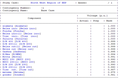
Figure 9

Figure 9. Each bus's voltage violations in the base.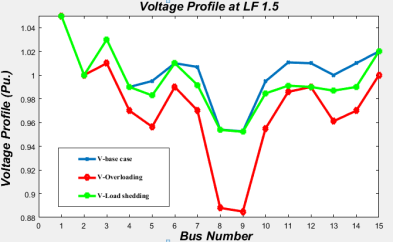
Figure 10

Figure 10. Magnitudes of voltage (PU) base case, load, and Shedd after LF 1.5.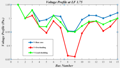
Figure 11

Figure 11. Magnitudes of voltage (PU) base case, load, and Shedd at LF 1.75.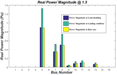
Figure 12

Figure 12. Load power (PU) base case, load, and Shedd at LF1.5.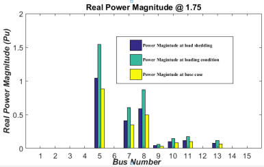
Figure 13

Figure 13. Load power (PU)base case, load, and Shedd at LF 1.75.

Table 1

Table 1. Alarm and security limits.Alarm and security limits.
Table 2

Table 2. Bus voltage of the 15 bus system in Normal, during contingency (Load Factor 1.5), and after load shed.Bus voltage of the 15 bus system in Normal, during contingency (Load Factor 1.5), and after load shed.
Table 3

Table 3. Bus voltage of 15 bus systems in Normal, during contingency (1.75 Load Factor), and after load shed.Bus voltage of 15 bus systems in Normal, during contingency (1.75 Load Factor), and after load shed.
Table 4

Table 4. Real power of the load bus in normal, during contingency (1.5 Load Factor), and after load shed.Real power of the load bus in normal, during contingency (1.5 Load Factor), and after load shed.
Table 5

Table 5. Real power of the load bus in normal, during contingency (1.75 Load factor), and after load shed.Real power of the load bus in normal, during contingency (1.75 Load factor), and after load shed.

Plain Text BibTeX RIS

APA Style

Geremew, M. S., Workie, Y. G., Kamau, J. N., Saoke, C. O., Aeggegn, D. B., et al. (2026). Optimized Load Shedding for Voltage Resilience in Ethiopia's Power Grid. American Journal of Electrical Power and Energy Systems, 15(1), 1-13. https://doi.org/10.11648/j.epes.20261501.11

Copy | Download

ACS Style

Geremew, M. S.; Workie, Y. G.; Kamau, J. N.; Saoke, C. O.; Aeggegn, D. B., et al. Optimized Load Shedding for Voltage Resilience in Ethiopia's Power Grid. Am. J. Electr. Power Energy Syst. 2026, 15(1), 1-13. doi: 10.11648/j.epes.20261501.11

Copy | Download

AMA Style

Geremew MS, Workie YG, Kamau JN, Saoke CO, Aeggegn DB, et al. Optimized Load Shedding for Voltage Resilience in Ethiopia's Power Grid. Am J Electr Power Energy Syst. 2026;15(1):1-13. doi: 10.11648/j.epes.20261501.11

Copy | Download

@article{10.11648/j.epes.20261501.11,
  author = {Mebratu Sintie Geremew and Yalew Gebru Workie and Joseph Ngugi Kamau and Churchill Otieno Saoke and Dessalegn Bitew Aeggegn and Gedef Yigalem Sharie},
  title = {Optimized Load Shedding for Voltage Resilience in Ethiopia's Power Grid},
  journal = {American Journal of Electrical Power and Energy Systems},
  volume = {15},
  number = {1},
  pages = {1-13},
  doi = {10.11648/j.epes.20261501.11},
  url = {https://doi.org/10.11648/j.epes.20261501.11},
  eprint = {https://article.sciencepublishinggroup.com/pdf/10.11648.j.epes.20261501.11},
  abstract = {This study deals with the essential operational challenges of voltage instability in the Northwest Ethiopian transmission network (NETN), which is a rapidly growing energy demand. An intelligent voltage load-shedding framework, Particle Swarm Optimization, was used for the multi-objective function under contingency scenarios. The proposed method, tested on NETN, comprising 15 buses, 15 lines, two generators, and three external grids, was used to analyze the grid behavior under significant load escalation (50% and 75% increase). The results indicated severe voltage drops at critical buses, notably Metema and Gondar (Metema’s voltage declined from 0.978 p.u. to 0.8638 p.u. at 75% overload). The proposed algorithm combines voltage sensitivity indices with dynamic load-shedding logic to determine the exact place & magnitude of real power changes. PSO-based optimization simultaneously minimizes active power curtailment while maximizing voltage profile recovery. Upon activation, the strategy restored bus voltages to secure levels (Metema up to 0.9538 p.u.) with precise bus-specific shedding of real power. This method effectively and rapidly transitions the system from an emergency to a normal state with minimal load loss. In contrast to traditional approaches, this comprehensive method explores feasibility in near real-time and guarantees system-wide coordination, providing a cost-effective solution for enhancing reliability in developing power systems across various uncertainty and stress conditions. These findings provide an innovative and practical foundation for enhancing the voltage stability.},
 year = {2026}
}

Copy | Download